Category: Environment

By Brett Scheffers, University of Florida and James Watson, The University of Queensland.

More than a dozen authors from different universities and nongovernmental organizations around the world have concluded, based on an analysis of hundreds of studies, that almost every aspect of life on Earth has been affected by climate change.

In more scientific parlance, we found in a paper published in Science that genes, species and ecosystems now show clear signs of impact. These responses to climate change include species’ genome (genetics), their shapes, colors and sizes (morphology), their abundance, where they live and how they interact with each other (distribution). The influence of climate change can now be detected on the smallest, most cryptic processes all the way up to entire communities and ecosystems.

Some species are already beginning to adapt. The color of some animals, such as butterflies, is changing because dark-colored butterflies heat up faster than light-colored butterflies, which have an edge in warmer temperatures. Salamanders in eastern North America and cold-water fish are shrinking in size because being small is more favorable when it is hot than when it is cold. In fact, there are now dozens of examples globally of cold-loving species contracting and warm-loving species expanding their ranges in response to changes in climate.

All of these changes may seem small, even trivial, but when every species is affected in different ways these changes add up quickly and entire ecosystem collapse is possible. This is not theoretical: Scientists have observed that the cold-loving kelp forests of southern Australia, Japan and the northwest coast of the U.S. have not only collapsed from warming but their reestablishment has been halted by replacement species better adapted to warmer waters.

Flood of insights from ancient flea eggs

Researchers are using many techniques, including one called resurrection ecology, to understand how species are responding to changes in climate by comparing the past to current traits of species. And a small and seemingly insignificant organism is leading the way.

One hundred years ago, a water flea (genus Daphnia), a small creature the size of a pencil tip, swam in a cold lake of the upper northeastern U.S. looking for a mate. This small female crustacean later laid a dozen or so eggs in hopes of doing what Mother Nature intended – that she reproduce.

Her eggs are unusual in that they have a tough, hardened coat that protects them from lethal conditions such as extreme cold and droughts. These eggs have evolved to remain viable for extraordinary periods of time and so they lay on the bottom of the lake awaiting the perfect conditions to hatch.

Now fast forward a century: A researcher interested in climate change has dug up these eggs, now buried under layers of sediment that accumulated over the many years. She takes them to her lab and amazingly, they hatch, allowing her to show one thing: that individuals from the past are of a different architecture than those living in a much hotter world today. There is evidence for responses at every level from genetics to physiology and up through to community level.

By combining numerous research techniques in the field and in the lab, we now have a definitive look at the breadth of climate change impacts for this animal group. Importantly, this example offers the most comprehensive evidence of how climate change can affect all processes that govern life on Earth.

From genetics to dusty books

The study of water fleas and resurrection ecology is just one of many ways that thousands of geneticists, evolutionary scientists, ecologists and biogeographers around the world are assessing if – and how – species are responding to current climate change.

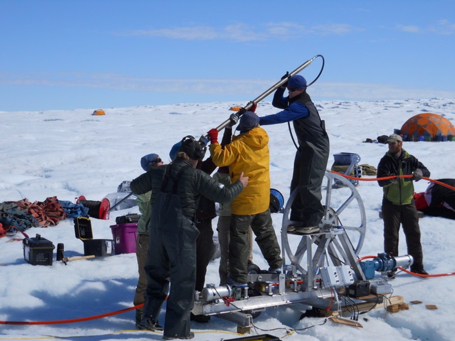
Other state-of-the-art tools include drills that can sample gases trapped several miles beneath the Antarctic ice sheet to document past climates and sophisticated submarines and hot air balloons that measure the current climate.

Researchers are also using modern genetic sampling to understand how climate change is influencing the genes of species, while resurrection ecology helps understand changes in physiology. Traditional approaches such as studying museum specimens are effective for documenting changes in species morphology over time.

Some rely on unique geological and physical features of the landscape to assess climate change responses. For example, dark sand beaches are hotter than light sand beaches because black color absorbs large amounts of solar radiation. This means that sea turtles breeding on dark sand beaches are more likely to be female because of a process called temperature dependent sex determination. So with higher temperatures, climate change will have an overall feminizing effect on sea turtles worldwide.

Wiping the dust off of many historical natural history volumes from the forefathers and foremothers of natural history, who first documented species distributions in the late 1800s and early 1900s, also provides invaluable insights by comparing historical species distributions to present-day distributions.

For example, Joseph Grinnell’s extensive field surveys in early 1900s California led to the study of how the range of birds there shifted based on elevation. In mountains around the world, there is overwhelming evidence that all forms of life, such as mammals, birds, butterflies and trees, are moving up towards cooler elevations as the climate warms.

How this spills over onto humanity

So what lessons can be taken from a climate-stricken nature and why should we care?

This global response occurred with just a 1 degree Celsius increase in temperature since preindustrial times. Yet the most sensible forecasts suggest we will see at least an increase of up to an additional 2-3 degrees Celsius over the next 50 to 100 years unless greenhouse gas emissions are rapidly cut.

All of this spells big trouble for humans because there is now evidence that the same disruptions documented in nature are also occurring in the resources that we rely on such as crops, livestock, timber and fisheries. This is because these systems that humans rely on are governed by the same ecological principles that govern the natural world.

Examples include reduced crop and fruit yields, increased consumption of crops and timber by pests and shifts in the distribution of fisheries. Other potential results include the decline of plant-pollinator networks and pollination services from bees.

Further impacts on our health could stem from declines in natural systems such as coral reefs and mangroves, which provide natural defense to storm surges, expanding or new disease vectors and a redistribution of suitable farmland. All of this means an increasingly unpredictable future for humans.

This research has strong implications for global climate change agreements, which aim to keep total warming to 1.5C. If humanity wants our natural systems to keep delivering the nature-based services we rely so heavily on, now is not the time for nations like the U.S. to step away from global climate change commitments. Indeed, if this research tells us anything it is absolutely necessary for all nations to up their efforts.

Humans need to do what nature is trying to do: recognize that change is upon us and adapt our behavior in ways that limit serious, long-term consequences.

Brett Scheffers, Assistant Professor, University of Florida and James Watson, Associate Professor, The University of Queensland

This article was originally published on The Conversation. Read the original article.

Now, Check Out:

• World set for hottest year on record: World Meteorological Organization
• Is global warming causing marine diseases to spread?
• Biofuels turn out to be a climate mistake – here’s why
• Series of NASA CubeSat Missions Will Take a Fresh Look at Planet Earth [Video]
• As climate change alters the oceans, what will happen to Dungeness crabs?

By Blair Trewin, World Meteorological Organization.

2016 is set to be the world’s hottest year on record. According to the World Meteorological Organization’s preliminary statement on the global climate for 2016, global temperatures for January to September were 0.88°C above the long-term (1961-90) average, 0.11°C above the record set last year, and about 1.2°C above pre-industrial levels.

While the year is not yet over, the final weeks of 2016 would need to be the coldest of the 21st century for 2016’s final number to drop below last year’s.

Record-setting temperatures in 2016 came as no real surprise. Global temperatures continue to rise at a rate of 0.10-0.15°C per decade, and over the five years from 2011 to 2015 they averaged 0.59°C above the 1961-1990 average.

Giving temperatures a further boost this year was the very strong El Niño event of 2015−16. As we saw in 1998, global temperatures in years where the year starts with a strong El Niño are typically 0.1-0.2°C warmer than the years either side of them, and 2016 is following the same script.

Almost everywhere was warm

Warmth covered almost the entire world in 2016, but was most significant in high latitudes of the Northern Hemisphere. Some parts of the Russian Arctic have been a remarkable 6-7°C above average for the year, while Alaska is having its warmest year on record by more than a degree.

Almost the whole Northern Hemisphere north of the tropics has been at least 1°C above average. North America and Asia are both having their warmest year on record, with Africa, Europe and Oceania close to record levels. The only significant land areas which are having a cooler-than-normal year are northern and central Argentina, and parts of southern Western Australia.

The warmth did not just happen on land; ocean temperatures were also at record high levels in many parts of the world, and many tropical coral reefs were affected by bleaching, including the Great Barrier Reef off Australia.

Greenhouse gas levels continued to rise this year. After global carbon dioxide concentrations reached 400 parts per million for the first time in 2015, they reached new record levels during 2016 at both Mauna Loa in Hawaii and Cape Grim in Australia.

On the positive side, the Antarctic ozone hole in 2016 was one of the smallest of the last decade; while there is not yet a clear downward trend in its size, it is at least not growing any more.

Global sea levels continue to show a consistent upward trend, although they have temporarily levelled off in the last few months after rising steeply during the El Niño.

Droughts and flooding rains

El Niño was over by May 2016 – but many of its effects are still ongoing.

Worst affected was southern Africa, which gets most of its rain during the Southern Hemisphere summer. Rainfall over most of the region was well below average in both 2014-15 and 2015-16.

With two successive years of drought, many parts are suffering badly with crop failures and food shortages. With the next harvests due early in 2017, the next couple of months will be crucial in prospects for recovery.

Drought is also strengthening its grip in parts of eastern Africa, especially Kenya and Somalia, and continues in parts of Brazil.

On the positive side, the end of El Niño saw the breaking of droughts in some other parts of the world. Good mid-year rains made their presence felt in places as diverse as northwest South America and the Caribbean, northern Ethiopia, India, Vietnam, some islands of the western tropical Pacific, and eastern Australia, all of which had been suffering from drought at the start of the year.

The world has also had its share of floods during 2016. The Yangtze River basin in China had its wettest April to July period this century, with rainfall more than 30% above average. Destructive flooding affected many parts of the region, with more than 300 deaths and billions of dollars in damage.

Europe was hard hit by flooding in early June, with Paris having its worst floods for more than 30 years.

In western Africa, the Niger River reached its highest levels for more than 50 years in places, although the wet conditions also had many benefits for the chronically drought-affected Sahel, and eastern Australia also had numerous floods from June onwards as drought turned to heavy rain.

Tropical cyclones are among nature’s most destructive phenomena, and 2016 was no exception. The worst weather related natural disaster of 2016 was Hurricane Matthew. Matthew reached category five intensity south of Haiti, the strongest Atlantic storm since 2007. It hit Haiti as a category 4 hurricane, causing at least 546 deaths, with 1.4 million people needing humanitarian assistance. The hurricane then went on to cause major damage in Cuba, the Bahamas and the United States.

Other destructive tropical cyclones in 2016 included Typhoon Lionrock, responsible for flooding in the Democratic People’s Republic of Korea which claimed at least 133 lives, and Cyclone Winston, which killed 44 people and caused an estimated US$1.4 billion damage in Fiji’s worst recorded natural disaster.

Arctic sea ice extent was well-below average all year. It reached a minimum in September of 4.14 million square kilometres, the equal second smallest on record, and a very slow autumn freeze-up so far means that its extent is now the lowest on record for this time of year.

In the Antarctic, sea ice extent was fairly close to normal through the first part of the year but has also dropped well below normal over the last couple of months, as the summer melt has started unusually early.

It remains to be seen what impact the summer of 2016 has had on the mountain glaciers of the Northern Hemisphere.

While 2016 has been an exceptional year by current standards, the long-term warming trends mean there will be more years like it to come. Recent research has shown that global average temperatures which are record-breaking now are likely to become the norm within the next couple of decades.

Blair Trewin, Lead author, 2016 WMO Global Statement on the Status of the Global Climate, World Meteorological Organization

This article was originally published on The Conversation. Read the original article.

Now, Check Out:

• August Marks Month 16 of Record-Breaking Warm Global Temperatures
• Arctic Sea Ice Minimum Ties Record for Lowest Coverage [Video]
• Scientist at work: Tracking melt water under the Greenland ice sheet
• The oceans are full of plastic, but why do seabirds eat it?
• Why the current plan to save the endangered vaquita porpoise won’t work

By Andrew Frederick Johnson, University of California, San Diego.

With fewer than 60 individuals left, the world’s smallest porpoise, the vaquita marina (Phocoena sinus), continues to balance on the edge of extinction. Constant pressures from conservation groups have lead to a two-year emergency gillnet ban, which will end in May 2017, and government-led efforts are now pushing fishers to use gear that won’t threaten the vaquita through bycatch.

Despite these steps, in a new study my colleagues and I warn that unless further big changes are made in the Upper Gulf of California, Mexico, we may soon be saying goodbye to this charismatic little animal.

The history of vaquita conservation is long and convoluted. It has been characterized by intermittent top-down management interventions that have often had little more than short-term outlooks. These have perpetuated the decline of the vaquita population, which is now estimated to contain less than 25 reproductively mature females.

The new Conservation Letters study describes how the gillnet ban now in effect, and the introduction of new trawl gear may address the immediate problem of vaquita bycatch but even taken together, they will likely be yet another short-term – and, most likely, ineffective – attempt to pull the vaquita back from the brink of extinction.

Switching gears

Gillnets sit in midwater and are made of fine line, which is difficult to see in the Upper Gulf’s murky waters. Similar to almost all cetacean bycatch, vaquita are unable to free themselves once entangled and risk being drowned while held under water.

Trawl gear is an alternative that reduces the risk of bycatch. These heavy gears are towed along the seafloor catching any animal not quick enough to outswim the mouth of the approaching net. The mouth of the net is much smaller than the area of a gillnet, which reduces the effective catch area that poses a risk to the vaquita. Also, the use of trawl gear is noisy, more easily visible and therefore more easily avoidable than gillnets for cetacean species.

But this alternative is more expensive. After accounting for lower catch rates, higher fuel expenditure and the cost of the switch from gillnets to trawls, we estimated that an annual subsidy of at least US$8.5 million would be needed to compensate fishers in the Upper Gulf for loss of employment and earnings. Long term, the economic losses from the new management interventions could have one or two side effects: 1) a reliance on subsidies and/or 2) increased illegal fishing activities.

What’s more, an endangered yet highly prized fish is caught in these waters with gillnets. Swim bladders known as buche from the endangered totoaba (Totoaba macdonali) can sell for tens to hundreds of thousands of dollars per kilo, depending on the size of the bladder and the demand of the Chinese market. This “aquatic cocaine” complicates the plight of the vaquita because illegal fishing to catch the totoaba pose a risk to the few vaquita that remain.

There are also significant ecological risks to the new management plan. The impacts of trawl gear to seafloor species are significantly greater than those posed by gillnets because they are dragged along sea floors, reducing productivity in many shelf sea ecosystems and negatively affecting community compositions and diversity. In just 26 days of gear testing in the Upper Gulf prior to the the gillnet ban, 30 percent, or 2,819 square kilomters (1,715 square miles), of the Upper Gulf biosphere reserve’s total area was scoured by the new trawl gears. Longer term, we warn in our study this could have severely detrimental consequences for the health of the Upper Gulf marine ecosystem.

Community involvement

My colleagues and I believe there is little use in pointing the finger of blame at this point, as seems to be the case in many articles discussing the fight for the vaquita. Instead, the vaquita situation urgently needs a new way of thinking, a paradigm shift.

Consistent exclusion of fishers from the design of management plans, typically driven by conservation groups and implemented by the government, has led to polarized opinions and a large divide between what should be a close collaboration between fishers and conservation agencies. Rushed, short-sighted management must be replaced by longer-term goals that involve local communities and address conservation challenges associated with both the vaquita and the totoaba.

Community support of management measures, in particular, seems essential for long-term success in conservation stories. We recommend that the local communities in the Upper Gulf require external investment. Specifically, the development of infrastructure, such as road networks to connect fishers to new markets and processing facilities, would benefit the current situation by providing new employment opportunities as well as increased returns on ever dwindling fish catches.

Education is also key. This should include programs to educate fishers in the consequences of unsustainable fisheries practices, techniques to help add value to their catches and alternative livelihoods to fishing such as tourism or potential service industry employment.

At present there are few employment alternatives for fishers in the Upper Gulf. Often, men are recruited into the fishery as young as 15 and the common story of “once a fisher, always a fisher” prevails. We highlight that an investment in education could both help promote marine stewardship as fishers better understand the longer-term consequences of current fisheries practices. It could also provide the younger generation with the training to build new business or follow paths in higher education instead of joining the local fisheries.

As with many of the world’s ecological problems, overcapacity seems to be key. In the case of the upper Gulf fisheries, too many people are catching too many fish from finite stocks. Continued overexploitation of any natural resource ultimately means communities risk destroying the finite natural resources they depend on.

To put it simply, communities in the Upper Gulf of California need help to reduce both the number of fishers currently fishing and the number of future fishers entering the fisheries. This will help promote alternative, nonextractive activities in order to alleviate the impacts that current fisheries practices have on fish stocks, the vaquita and, with the new trawl gear intervention, sea floor habitats.

Another band-aid

A meeting in late July of this year between Presidents Obama and Peña Nieto concluded with a tentative proposal for a permanent extension of the Upper Gulf’s gillnet ban and a crack down on the totoaba trade. Although eliminating vaquita bycatch is crucial for the species’ survival, ignoring economic losses, local livelihoods and new ecological problems related to trawl impacts, the Mexican government may have missed the point again.

With one foot of the vaquita firmly in the grave, now does not seem to be the time to make somewhat incomplete decisions regarding the survival of the vaquita, the health of the Upper Gulf of California’s ecosystem and the social well being of the families that live in this remote area of Mexico.

Andrew Frederick Johnson, Postdoctoral Researcher of Marine Biology at Scripps Insitution of Oceanography, University of California, San Diego

This article was originally published on The Conversation. Read the original article.

Now, Check Out:

• How many genes does it take to make a person?
• Yoshinori Ohsumi – a deserving winner of the Nobel Prize for physiology or medicine
• Can great apes read your mind? [Videos]
• Scientist at work: Tracking melt water under the Greenland ice sheet
• Deepwater Horizon: scientists are still trying to unravel mysteries of the spill

By Tony Gutierrez, Heriot-Watt University.

The film Deepwater Horizon, starring Mark Wahlberg, captures the chaos and drama that ensued after the massive fireball that engulfed the oil rig of the same name in 2011, which killed 11 people and injured many others. The film dramatises the gruesome ordeal which saw more than 100 crew members battle to survive the inferno of sweltering heat and mayhem.

But the scientific frenzy that followed in the ensuing months was almost as dramatic. And now, just over six years on, there is still much that science has yet to uncover about the spill in the hope of preparing us for the next big one.

Where, for instance, did all the oil actually end up? And what did all the chemicals dumped in the ocean to break up the oil do to the marine life that survived the spill? These questions and more remain unanswered.

The Deepwater Horizon disaster stands in the record books as the largest oil spill in US history. Following the blowout on April 20, 2010, 4.1m barrels (0.7m tonnes) of crude oil leaked into the Gulf of Mexico over a period of almost three months. Only the 1979 Ixtoc-I oil spill, also in the Gulf of Mexico, ranks in the same league.

It was a particularly complex and challenging spill to deal with and study, for several reasons. The exploratory well below Deepwater Horizon was itself an extraordinary engineering feat, the deepest the oil and gas industry had ever drilled in the ocean. The spill occurred about 1.5km below the sea surface, again, the deepest in history. And, because it occurred in such deep water, a good chunk of the oil didn’t rise to the surface as in a usual spill – instead, an unprecedented “oil plume” formed below the surface and lingered there for months.

Rarely has a human-made disaster ever stopped the clock on the research programmes of so many scientists in a nation. Scientists from universities and government-funded agencies all over the US put their work on hold in order to turn their attention to Deepwater Horizon. More than 400 scientific peer-reviewed papers have now been published on the spill, and they’ve revealed a lot of important information.

Within weeks of the spill occurring scientists reported the formation of a massive plume of crude oil a kilometre below the surface that stretched for about 30km and was 300 metres high. It was difficult to track, but nonetheless was intensively studied as researchers realised they had a unique opportunity. Within this oil cloud, scientists also showed that certain types of oil-degrading bacteria had bloomed and that these microbes played a fundamental role in degrading the oil in the deep as well as on sea surface oil slicks of the Gulf.

Research also demonstrated that the oil caused lasting damage to Gulf coast marshes, and that it affected the spawning habitat of Bluefin tuna along the south-east coast of North America.

After the spill, scientists noticed huge quantities of lightly-coloured mucus-like particles or blobs on the sea surface in and around the spill site. These “blobs” could be barely big enough to see, or large enough to fit in your hand. Nothing of this magnitude had been observed before, although there is evidence that similar particles had also formed during the Ixtoc-I spill.

It turned out this was caused by oil sticking to “marine snow” – small specs of dead plankton, bacteria, the mucus they produce, and so on, that clump together near the surface and then fall through the ocean just as real snow falls through the sky. As this “marine oil snow” sank through the water, it took with it a large proportion of the oil from the sea surface and eventually settled on the seabed.

Mysteries remain

Just over six years later, scientists are still trying to understand the full extent of Deepwater Horizon’s impacts on the seabed, beaches and marshes of the Gulf of Mexico. This is actually not a great length of time for science to fully understand a massive and complex spill like this, so its no wonder that some things still remain a mystery.

We know that a lot of the oil from the leaky well that reached the surface made it to the Gulf coast, for instance, and caused acute damage to coastal ecosystems. But we do not know where the deepwater oil plume ended up or what its impact was. Likewise we still don’t know the longer-term impact of the expansive surface oil slicks in the Gulf.

We also need to better understand the impacts of the chemicals that were used to disperse the oil after the spill. Around 7m litres of a dispersant called Corexit was sprayed into the sea by planes or ships. However, given oil dispersant is essentially strong household soap, these chemicals posed a problem for coral and other marine organisms in the Gulf, including the same oil-degrading bacteria that are so critical in the natural bio-degradation process after the spill. Research shows the dispersant used was probably counter-productive.

There is still much to be learnt about what Corexit and other dispersants do to marine life in the longer term. This is important as dispersants are a first line of response to combat oil spills at sea.

Research on the spill is likely to continue for the next few decades. With many oil and gas reservoirs coming to the end of their lives the industry is expanding into the Arctic and other challenging environments, and exploring ever-deeper ocean waters. Another spill like Deepwater Horizon cannot be discounted. What science has already uncovered, and what it will do in years to come, is crucial and should help to better prepare us to deal with the next big one.

Tony Gutierrez, Associate Professor of Microbiology, Heriot-Watt University

This article was originally published on The Conversation. Read the original article.

Now, Check Out:

• Can great apes read your mind? [Videos]
• Biofuels turn out to be a climate mistake – here’s why
• Scientist at work: Tracking melt water under the Greenland ice sheet
• [Video] Underwater robots help scientists see where marine larvae go and how they get there
• Alligators Are Ancient: New Studies Show They Haven’t Evolved for Over 8 Million Years

By John DeCicco, University of Michigan.

Ever since the 1973 oil embargo, U.S. energy policy has sought to replace petroleum-based transportation fuels with alternatives. One prominent option is using biofuels, such as ethanol in place of gasoline and biodiesel instead of ordinary diesel.

Transportation generates one-fourth of U.S. greenhouse gas emissions, so addressing this sector’s impact is crucial for climate protection.

Many scientists view biofuels as inherently carbon-neutral: they assume the carbon dioxide (CO2) plants absorb from the air as they grow completely offsets, or “neutralizes,” the CO2 emitted when fuels made from plants burn. Many years of computer modeling based on this assumption, including work supported by the U.S. Department of Energy, concluded that using biofuels to replace gasoline significantly reduced CO2 emissions from transportation.

Our new study takes a fresh look at this question. We examined crop data to evaluate whether enough CO2 was absorbed on farmland to balance out the CO2 emitted when biofuels are burned. It turns out that once all the emissions associated with growing feedstock crops and manufacturing biofuel are factored in, biofuels actually increase CO2 emissions rather than reducing them.

Biofuel boom, climate blunder

Federal and state policies have subsidized corn ethanol since the 1970s, but biofuels gained support as a tool for promoting energy independence and reducing oil imports after the September 11, 2001 attacks. In 2005 Congress enacted the Renewable Fuel Standard, which required fuel refiners to blend 7.5 billion gallons of ethanol into gasoline by 2012. (For comparison, in that year Americans used 133 billion gallons of gasoline.)

In 2007 Congress dramatically expanded the RFS program with support from some major environmental groups. The new standard more than tripled annual U.S. renewable fuel consumption, which rose from 4.1 billion gallons in 2005 to 15.4 billion gallons in 2015.

Our study examined data from 2005-2013 during this sharp increase in renewable fuel use. Rather than assuming that producing and using biofuels was carbon-neutral, we explicitly compared the amount of CO2 absorbed on cropland to the quantity emitted during biofuel production and consumption.

Existing crop growth already takes large amounts of CO2 out of the atmosphere. The empirical question is whether biofuel production increases the rate of CO2 uptake enough to fully offset CO2 emissions produced when corn is fermented into ethanol and when biofuels are burned.

Most of the crops that went into biofuels during this period were already being cultivated; the main change was that farmers sold more of their harvest to biofuel makers and less for food and animal feed. Some farmers expanded corn and soybean production or switched to these commodities from less profitable crops.

But as long as growing conditions remain constant, corn plants take CO2 out of the atmosphere at the same rate regardless of how the corn is used. Therefore, to properly evaluate biofuels, one must evaluate CO2 uptake on all cropland. After all, crop growth is the CO2 “sponge” that takes carbon out of the atmosphere.

When we performed such an evaluation, we found that from 2005 through 2013, cumulative carbon uptake on U.S. farmland increased by 49 teragrams (a teragram is one million metric tons). Planted areas of most other field crops declined during this period, so this increased CO2 uptake can be largely attributed to crops grown for biofuels.

Over the same period, however, CO2 emissions from fermenting and burning biofuels increased by 132 teragrams. Therefore, the greater carbon uptake associated with crop growth offset only 37 percent of biofuel-related CO2 emissions from 2005 through 2013. In other words, biofuels are far from inherently carbon-neutral.

Carbon flows and the ‘climate bathtub’

This result contradicts most established work on biofuels. To understand why, it is helpful to think of the atmosphere as a bathtub that is filled with CO2 instead of water.

Many activities on Earth add CO2 to the atmosphere, like water flowing from a faucet into the tub. The largest source is respiration: Carbon is the fuel of life, and all living things “burn carbs” to power their metabolisms. Burning ethanol, gasoline or any other carbon-based fuel opens up the CO2 “faucet” further and adds carbon to the atmosphere faster than natural metabolic processes.

Other activities remove CO2 from the atmosphere, like water flowing out of a tub. Before the industrial era, plant growth absorbed more than enough CO2 to offset the CO2 that plants and animals respired into the atmosphere.

Today, however, largely through fossil fuel use, we are adding CO2 to the atmosphere far more rapidly than nature removes it. As a result, the CO2 “water level” is rapidly rising in the climate bathtub.

When biofuels are burned, they emit roughly the same the amount of CO2 per unit of energy as petroleum fuels. Therefore, using biofuels instead of fossil fuels does not change how quickly CO2 flows into the climate bathtub. To reduce the buildup of atmospheric CO2 levels, biofuel production must open up the CO2 drain – that is, it must speed up the net rate at which carbon is removed from the atmosphere.

Growing more corn and soybeans has opened the CO2 uptake “drain” a bit more, mostly by displacing other crops. That’s especially true for corn, whose high yields remove carbon from the atmosphere at a rate of two tons per acre, faster than most other crops.

Nevertheless, expanding production of corn and soybeans for biofuels increased CO2 uptake only enough to offset 37 percent of the CO2 directly tied to biofuel use. Moreover, it was far from enough to offset other GHG emissions during biofuel production from sources including fertilizer use, farm operations and fuel refining. Additionally, when farmers convert grasslands, wetlands and other habitats that store large quantities of carbon into cropland, very large CO2 releases occur.

Mistaken modeling

Our new study has sparked controversy because it contradicts many prior analyses. These studies used an approach called lifecycle analysis, or LCA, in which analysts add up all of the GHG emissions associated with producing and using a product. The result is popularly called the product’s “carbon footprint.”

The LCA studies used to justify and administer renewable fuel policies evaluate only emissions – that is, the CO2 flowing into the air – and failed to assess whether biofuel production increased the rate at which croplands removed CO2 from the atmosphere. Instead, LCA simply assumes that because energy crops such as corn and soybeans can be regrown from one year to the next, they automatically remove as much carbon from the atmosphere as they release during biofuel combustion. This significant assumption is hard-coded into LCA computer models.

Unfortunately, LCA is the basis for the RFS as well as California’s Low-Carbon Fuel Standard, a key element of that state’s ambitious climate action plan. It is also used by other agencies, research institutions and businesses with an interest in transportation fuels.

I once accepted the view that biofuels were inherently carbon-neutral. Twenty years ago I was lead author of the first paper proposing use of LCA for fuel policy. Many such studies were done, and a widely cited meta-analysis published in Science in 2006 found that using corn ethanol significantly reduced GHG emissions compared to petroleum gasoline.

However, other scholars raised concerns about how planting vast areas with energy crops could alter land use. In early 2008 Science published two notable articles. One described how biofuel crops directly displaced carbon-rich habitats, such as grasslands. The other showed that growing crops for biofuel triggered damaging indirect effects, such as deforestation, as farmers competed for productive land.

LCA adherents made their models more complex to account for these consequences of fuel production. But the resulting uncertainties grew so large that it became impossible to determine whether or not biofuels were helping the climate. In 2011 a National Research Council report on the RFS concluded that crop-based biofuels such as corn ethanol “have not been conclusively shown to reduce GHG emissions and might actually increase them.”

These uncertainties spurred me to start deconstructing LCA. In 2013, I published a paper in Climatic Change showing that the conditions under which biofuel production could offset CO2 were much more limited than commonly assumed. In a subsequent review paper I detailed the mistakes made when using LCA to evaluate biofuels. These studies paved the way for our new finding that in the United States, to date, renewable fuels actually are more harmful to the climate than gasoline.

It is still urgent to mitigate CO2 from oil, which is the largest source of anthropogenic CO2 emissions in the United States and the second-largest globally after coal. But our analysis affirms that, as a cure for climate change, biofuels are “worse than the disease.”

Reduce and remove

Science points the way to climate protection mechanisms that are more effective and less costly than biofuels. There are two broad strategies for mitigating CO2 emissions from transportation fuels. First, we can reduce emissions by improving vehicle efficiency, limiting miles traveled or substituting truly carbon-free fuels such as electricity or hydrogen.

Second, we can remove CO2 from the atmosphere more rapidly than ecosystems are absorbing it now. Strategies for “recarbonizing the biosphere” include reforestation and afforestation, rebuilding soil carbon and restoring other carbon-rich ecosystems such as wetlands and grasslands.

These approaches will help to protect biodiversity – another global sustainability challenge – instead of threatening it as biofuel production does. Our analysis also offers another insight: Once carbon has been removed from the air, it rarely makes sense to expend energy and emissions to process it into biofuels only to burn the carbon and re-release it into the atmosphere.

John DeCicco, Research Professor, University of Michigan

This article was originally published on The Conversation. Read the original article.

Now, Check Out:

• [Video] Underwater robots help scientists see where marine larvae go and how they get there
• Here’s Evidence that a Massive Collision Formed the Moon
• Genetic studies reveal diversity of early human populations – and pin down when we left Africa
• Why teen brains need later school start time
• Scientist at work: Tracking melt water under the Greenland ice sheet

According to a new report from the National Oceanic and Atmospheric Adminstration (NOAA), August 2016 was the 16th consecutive record-breaking month in a row for warmer temperatures around the globe for planet Earth, across all 7 temperature measures that have been used for many decades to measure global temperatures. These measurements include land, sea, and atmospheric temperatures as well as sea ice measurements. Additionally, the global temperature for August is the highest in 176 years of record keeping, surpassing August of 2014.

 

A companion announcement issued simultaneously by the NASA Earth Observatory reports that August 2016 was the warmest August in 136 years of modern record-keeping, according to a monthly analysis of global temperatures by scientists at NASA’s Goddard Institute for Space Studies (GISS).

Although the seasonal temperature cycle typically peaks in July, August 2016 wound up tied with July 2016 for the warmest month ever recorded. August 2016’s temperature was 0.16 degrees Celsius warmer than the previous warmest August (2014). The month also was 0.98 degrees Celsius warmer than the mean August temperature from 1951-1980.

“Monthly rankings, which vary by only a few hundredths of a degree, are inherently fragile,” said GISS Director Gavin Schmidt. “We stress that the long-term trends are the most important for understanding the ongoing changes that are affecting our planet.” Those long-term trends are apparent in the plot of temperature anomalies above.

The record warm August continued a streak of 11 consecutive months (dating to October 2015) that have set new monthly temperature records. The analysis by the GISS team is assembled from publicly available data acquired by about 6,300 meteorological stations around the world, ship- and buoy-based instruments measuring sea surface temperature, and Antarctic research stations. The modern global temperature record begins around 1880 because previous observations didn’t cover enough of the planet.

Sources: News and data releases from NOAA and the NASA Earth Observatory.

Featured Image Credit: NASA Earth Observatory

Now, Check Out:

• Arctic Sea Ice Minimum Ties Record for Lowest Coverage [Video]
• Overcooling and overheating buildings emits as much carbon as four million cars
• As climate change alters the oceans, what will happen to Dungeness crabs?
• There are bright spots among the world’s coral reefs – the challenge is to learn from them
• These Coral Reefs Have Become ‘Ghost Towns’ in Just a Few Months [Video]

By Eric Williams, Rochester Institute of Technology.

Six years ago, Phoenix lay burning in the sun one day. It was 110 degrees Fahrenheit and I was the only person foolish enough to be out walking instead of moving by air-conditioned car. Arriving hot and parched at a bookstore, I opened the doors to be greeted by a blast of arctic air.

The coffee shop in which I sat down felt like it was freezing. Other customers, dressed in light summer wear for Phoenix summers, were shivering. We all chatted about how cold it was, so I went over to the coffee shop manager to see if the thermostat could be changed. He agreed wholeheartedly it was entirely too cold but reported that the temperature was decided and controlled not by the branch, but at the national headquarters.

As many people know, this is an extreme example of a common experience. Americans often find themselves in a store or office that’s too cold in summer or too hot in winter.

Obviously one can’t find a temperature that will please everyone all the time, but if lots of people are dissatisfied, this is a double dose of nonsense: Energy being wasted to make people uncomfortable. This led to the questions that would guide my research: What are the thermostat settings in commercial buildings and why are they set there? How much energy is wasted in making people uncomfortable?

In the end, I was surprised at how big the impact of poor thermal management in buildings is on our country’s energy consumption.

Inefficiencies

Making progress on my research questions went on hold until I was situated in a less extreme environment than Phoenix – Rochester, New York – when I started working with Ph.D. candidate Lourdes Gutierrez, who quickly uncovered many interesting things. One is that 42 percent of workers report being dissatisfied with the temperature in their offices, with 14 percent being very dissatisfied. Thus, there is a widespread problem with thermal comfort. Curiously, there is much less information available as to what thermostat settings are and how they are decided.

Lourdes also realized thermostat settings should vary by season and location. An office worker in Minnesota, for example, will wear heavier clothes in winter than one in Florida, so the thermostat in Minnesota can be set at a lower temperature.

We went on to analyze the national potential for energy savings from changing thermostat settings, by bumping them up in summer and down in winter by an amount appropriate for the local climate.

The first step was to figure out what winter and summer thermostat settings would ensure comfort for least 80 percent of occupants in 14 different U.S. cities. Eighty percent satisfaction is a typical compromise used by experts in thermal comfort. One result of our analysis was that in winter the thermostat could be safely set at 68F (20 degrees Celsius) in Minneapolis, while in Miami 72F (22C) is a better choice, since Miami-ites will be dressed lighter.

Next, we used energy simulation models to calculate the change in energy use with these new thermostat settings, compared with the typical year-round setting of 70F (21C). Not all buildings are set year-round at 70F, but it is considered a typical figure. There are many types of commercial buildings; we decided to focus on office buildings and restaurants as important, but tractable, types.

Our results, recently published in “Sustainable Cities and Society,” showed that the new thermostat settings could reduce 2.5 percent of energy use in U.S. office buildings and restaurants. National savings on utility bills would total US$600 million.

If other types of commercial buildings such as hotels and stores get similar savings as offices and restaurants, revised thermostat settings would reduce national carbon emissions by 0.3 percent. These saved carbon emissions are equivalent to the carbon pollution generated by four million automobiles in a year. This isn’t going to save the world from climate change, but it is a heck of a lot of carbon to be reduced while saving money and making people more comfortable.

Better data and monitoring

Where to go from here? We don’t claim to have the final answer on what thermostat settings should be and how much energy could be saved, as it’s a complicated question and will vary by building.

But we do argue these results highlight the need to rethink thermostat settings in offices, stores, restaurants and other commercial buildings. Managers should investigate what thermostat settings will make their customers and employees comfortable, considering the local climate. Dress code also plays a role: The closer employee clothing fits the outdoor environment, the more energy can be saved from moving thermostat settings closer to ambient.

There are a number of other obvious steps for improving the comfort of people in buildings, while using less energy. Energy auditors can advise building managers as to how much they could save with different thermostat settings. Governments can be more active in collecting data on indoor temperatures and thermostat settings in commercial buildings. And to all you building occupants out there: If you find your office, store or restaurant too cold in summer or warm in winter, let management know about it.

Eric Williams, Associate Professor of Sustainability, Rochester Institute of Technology

This article was originally published on The Conversation. Read the original article.

Next, Check Out:

• As climate change alters the oceans, what will happen to Dungeness crabs?
• Arctic Sea Ice Minimum Ties Record for Lowest Coverage [Video]
• An official welcome to the Anthropocene epoch – but who gets to decide it’s here?
• Finding better ways to get hydrogen fuel from water
• Fracking and health: What we know from Pennsylvania’s natural gas boom